Population distributions and graphical output with privacy

Main article: Aggregation techniques

We have discussed probability distributions, either binned or continuous, in which each distribution was the result of a single source’s answer. We learned how to combine such distributions via Bayesian or averaging techniques. But another way to present respondents’ information is to simply transfer it to the top-most node and display it in a graphical or tabular form. The top node (the guy asking the question) then benefits from having all the information at a glance and can draw his own conclusions from it.

There are some privacy considerations to take into account when doing this, particularly that we don’t want to reveal each node’s trust value to the top-most node. So we’d want to aggregate the trust values as we roll up the results and subsequently use them to plug them into the Bayes eqn, a straight averaging, or trust-weighted averaging scheme.

Preserving privacy while calculating trust-modified probabilities

The math to calculate the Bayesian combinations or the averaged results is not any different than what we’ve done in the past although the procedures may vary slightly in order to preserve the privacy of Trust information.

In particular we want to ensure that we are aggregating trust values as we go along in order to hide the individual values. For the Bayesian combination we can apply the trust to each probability as we go along and generate a trust-modified probability (or probability distribution) for each node per Sapienza (https://ceur-ws.org/Vol-1664/w9.pdf) (or the augmented Sapienza method). No separate trust information is then conveyed for this case. For straight averaging, we can do the same. For trust-weighted averaging we can multiply trust values for each step together for each node and then add these together at the top node for the denominator.

Let’s do a simple example based on a tree with 10 nodes and 3 levels:

For the Sapienza modified trust (used in Bayes and simple averaging) we start at the bottom and work up (as we did previously). First we trust-modify the probabilities at Level 2 (the bottom).

${\textstyle P_{mod25}=P_{nom}+T(P-P_{nom})=0.5+0.9(0.6-0.5)=0.59}$

${\textstyle P_{mod26}=0.5+0.9(0.9-0.5)=0.86}$

${\textstyle P_{mod37}=0.5+0.9(0.55-0.5)=0.545}$

${\textstyle P_{mod38}=0.5+0.9(0.65-0.5)=0.635}$

${\textstyle P_{mod49}=0.5+0.9(0.7-0.5)=0.68}$

${\textstyle P_{mod410}=0.5+0.9(0.8-0.5)=0.77}$

For each node at Level 2 we can append the probabilities just found to those of the node’s themselves. We assume the nodes trust themselves (T=1) and thus need no modification.

${\textstyle P_{mod2}=[0.3,0.59,0.86]}$

${\textstyle P_{mod3}=[0.4,0.545,0.635]}$

${\textstyle P_{mod4}=[0.45,0.68,0.77]}$

These lists of probabilities are modified again by Trust (for the 1-2, 1-3, and 1-4 connection):

${\textstyle P_{mod12}=[0.5+0.9(0.3-0.5),0.5+0.9(0.59-0.5),0.5+0.9(0.86-0.5)]=[0.32,0.581,0.824]}$

${\textstyle P_{mod13}=[0.5+0.9(0.4-0.5),0.5+0.9(0.545-0.5),0.5+0.9(0.635-0.5)]=[0.41,0.5405,0.6215]}$

${\textstyle P_{mod14}=[0.5+0.9(0.45-0.5),0.5+0.9(0.68-0.5),0.5+0.9(0.77-0.5)]=[0.455,0.662,0.743]}$

These results can now be appended to Node 1 to form a complete list of all the probability answers:

${\textstyle P_{mod1}=[0.2,0.32,0.581,0.824,0.41,0.5405,0.6215,0.455,0.662,0.743]}$

The Bayesian combination of these is

${\textstyle P_{bay}=0.831}$

and the straight average is

${\textstyle P_{ave}=0.536}$

For the trust-weighted approach we proceed by tracking the numerator as the sum of the product of trust and probability and denominator as the sum of the trust. We are generally following what was done previously.

${\textstyle P_{2,numer}=0.3(1)+0.6(0.9)+0.9(0.9)=1.65}$

${\textstyle P_{2,denom}=1+0.9+0.9=2.8}$

at any point, the trust-weighted average is simply:

${\textstyle P_{2tave}={P_{2,numer} \over P_{2,denom}}={1.65 \over 2.8}=0.589}$

Now the same for nodes 3 and 4:

${\textstyle P_{3,numer}=0.4(1)+0.55(0.9)+0.65(0.9)=1.48}$

${\textstyle P_{3,denom}=1+0.9+0.9=2.8}$

${\textstyle P_{4,numer}=0.45(1)+0.7(0.9)+0.8(0.9)=1.8}$

${\textstyle P_{4,denom}=1+0.9+0.9=2.8}$

These numerators and denominators in turn are used to calculate the same for Node 1:

${\textstyle P_{1,numer}=0.2(1)+1.65(0.9)+1.48(0.9)+1.8(0.9)=4.637}$

${\textstyle P_{1,denom}=1+2.8(0.9)+2.8(0.9)+2.8(0.9)=8.56}$

The trust-weighted average is, as we’ve seen,

${\textstyle P_{1tave}={4.637 \over 8.56}=0.5417}$

Thus the combined probabilities, whether Bayesian or averaged, can be calculated at the top level without knowing the individual node’s trust values.

Viewing Population Data

Predicate Questions

Let’s return now to the list of probabilities we just calculated:

${\textstyle P_{mod1}=[0.2,0.32,0.581,0.824,0.41,0.5405,0.6215,0.455,0.662,0.743]}$

We can reorder them to reflect the Source numbers in the diagram above:

${\textstyle P_{mod1}=[0.2,0.32,0.41,0.455,0.581,0.824,0.5405,0.6215,0.662,0.743]}$

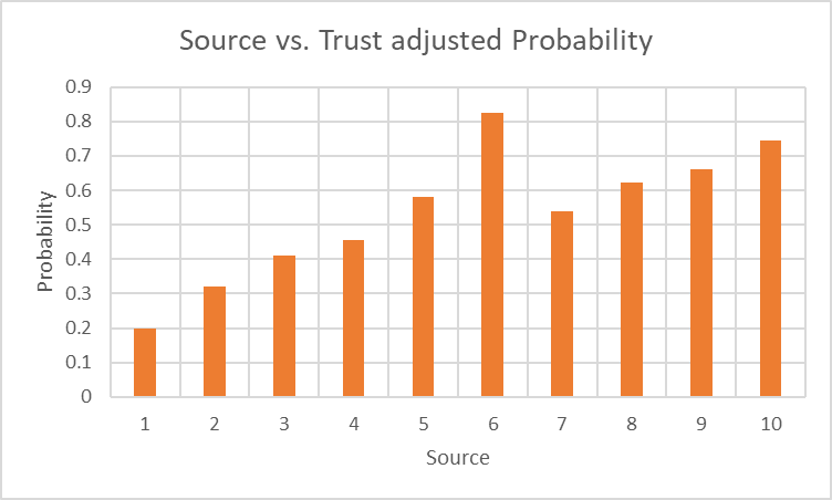
These results could simply be plotted as follows to get an idea of what everyone thinks. This will work if the population isn’t large and each individual result can be discerned:

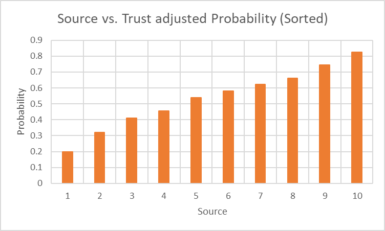
A sorted version of this could also be useful:

This shows a fairly even distribution of opinion, one for which it would be difficult to make a solid prediction.

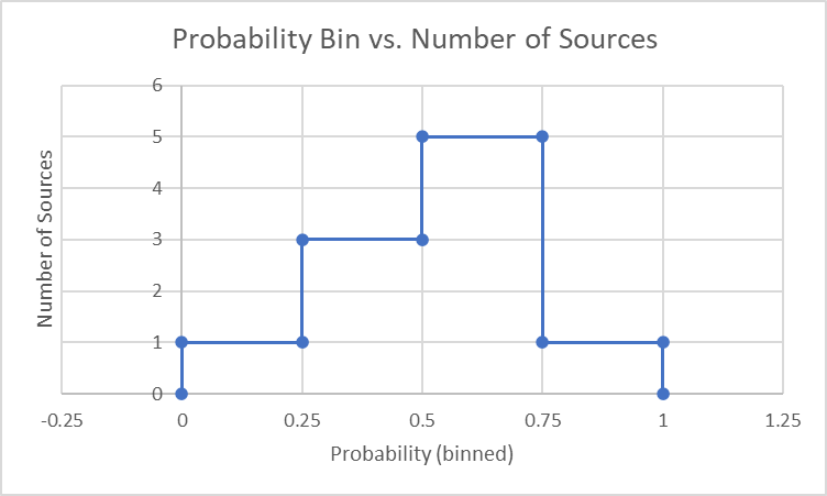
Let’s suppose the user finds the categories 0-0.25 (false), 0.25-0.5 (likely false), 0.5-0.75 (likely true), and 0.75-1 (true) significant and wants to bin results based on how many sources fall within each:

0.00-0.25: 1 node

0.25-0.50: 3 nodes

0.50-0.75: 5 nodes

0.75-1.00: 1 nodes

We can plot this result as follows:

From this it’s a little clearer that the 50%+ side of the graph is favored by a 6-4 vote. So if our bins get further reduced to two (True/False) the best answer to the question, from a vote-count perspective, is True.

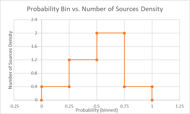
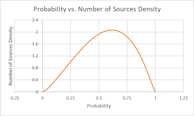
This can also be seen in terms of a probability distribution by dividing the y-axis values of the graph above by the number of samples (10) and the ${\textstyle \Delta x}$ (0.25).

If we were to imagine a much larger population, we might get a continuous distribution that looks something like this:

Non-Predicate Questions

The above model is for a predicate question, where only a single probability P is relevant (the other probability is 1-P). For questions with more than 2 answers, the respondent may answer with a probability distribution as we saw here. This doesn’t change the basic math and representation options but there are now more of them. Each probability graph would be plotted for each categorical option.

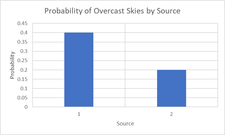
For example we could take the category of overcast skies from this discussion and plot the probabilities of the two respondents in the same way we did here:

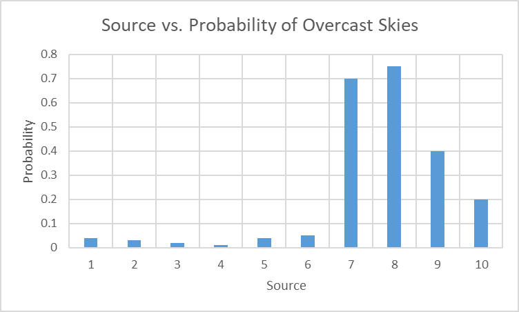
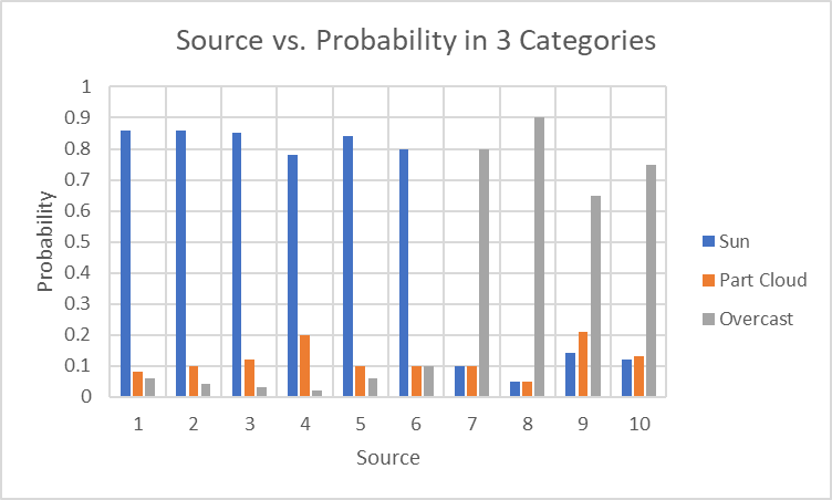
This isn’t a very interesting graph because there are only 2 respondents, but we could pretend there were 10:

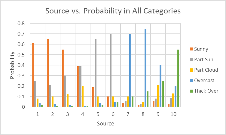
Given that this is only one category, we could plot similar results for the others as well: one for sunny, one for partly sunny, etc.

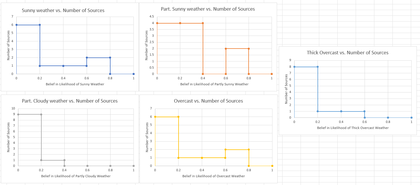
To plot the distribution of probability in each category we could establish a number of bins to represent Low (0-0.2), medium low (0.2-0.4), medium (0.4-0.6), medium high (0.6-0.8), and high (0.8-1.0) likelihood of each weather category (sunny, partly sunny, partly cloudy, overcast, thick overcast).

These graphs are difficult to generate conclusions from. Judging from the high number of sources at low probabilities (0-0.4) for each category, it is easy to conclude that a majority don’t believe in anything. Only 2 sources believe in sunny weather with a greater than 60% likelihood. One source believes in partly sunny weather with a greater than 60% likelihood. We also have 2 sources who believe in overcast weather with a greater than 60% likelihood, and no one who believes in thick overcast with greater than 60%. No one believes in partly cloudy (the middle option) with any degree of certainty. It is easy to conclude from this that there is no clear consensus about the weather tomorrow.

However, let’s bin things a little more coarsely by lumping the two sunny options together, leaving the partly cloudy option alone, and lumping the two overcast options together:

This changes things dramatically. Now we clearly see 6 sources who strongly believe in some form of sunny weather (either sunny or partly sunny). We see 4 who believe in some form of overcast weather.

Although not really needed, we can continue by creating a histogram with two bins for the x-axis, one for 0-0.5 and another for 0.5-1.

Again we see the 6 sources who believe in sunny weather and the 4 who believe in overcast weather.

This clearly shows a divided camp with a majority in favor of sunny weather. But it takes proper binning to achieve it and shows the importance of doing so. Needless to say, our users will need versatile graphical methods, in addition to the analytical tools we are providing.

One Use of Graphical Data: Finding Anomalous Sources

In this article a scenario was presented where someone gets an answer from a doctor with high trust and high confidence. Another answer from an acupuncturist comes in which lowers the overall confidence (in an averaging scheme). He argues that this seems wrong and proposes that we remove the acupuncturist’s opinion by taking the maximum calculated confidence and using that instead of an average. This is related to an earlier discussion about using the network to “find the expert”. In both these cases the user doesn’t really care about the consensus opinion but wants to find the one person with real knowledge of a possibly obscure subject (eg a medical question about a rare procedure). How would we go about locating that one person (or few people) if they are not a direct connection?

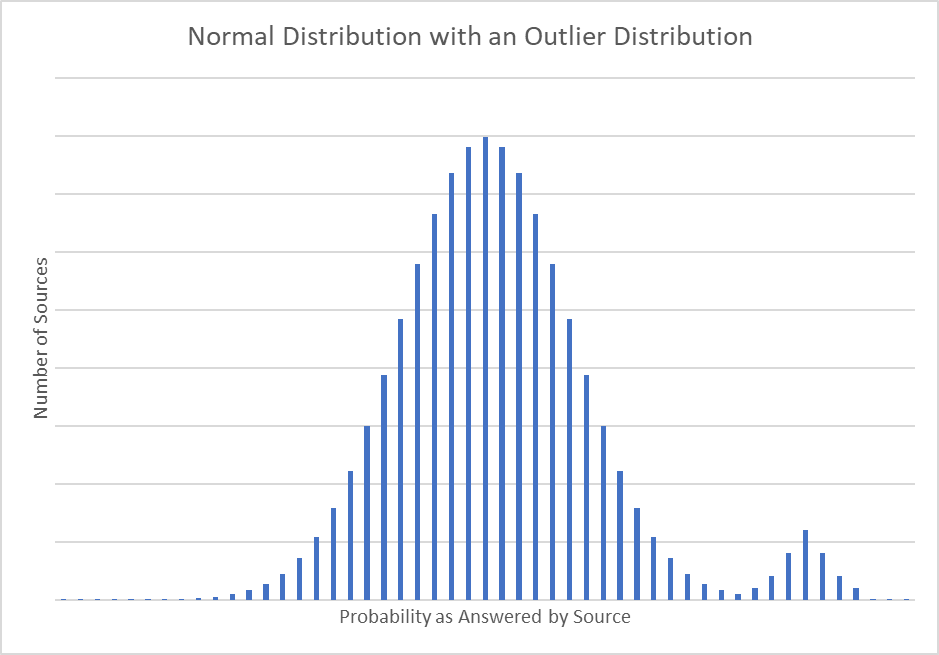
One way would be to find outliers in a histogram. This presumes that experts will often have their own strong opinion about a subject where the general public is far less sure. In the following graph, for instance, we have a normal distribution with a hump at one of the tails. The hump is another smaller group of people (experts) who answer the question with much high probability and are clustered to reflect a community with its own normally distributed data.

The user can easily identify this with a graphical distribution and then choose to drop the answers from the general public. Of course the hump may also reflect a cult which answers with high probability for superstitious reasons. In that case the user would drop the hump from consideration and go with the general public or perhaps find another hump which reflects the views of informed experts.

In either case the user would want the ability to know more about the cluster of anomalous data that he has located. He wouldn’t just know if they were a group of experts or charlatans unless he can find a way to get more information from them. One possible way to do that would be to establish the trust for the anomalous sources held by the community at large. A high level of trust would be a clue that the group is highly regarded as having expertise in a subject. We could then use Wang and Vassileva’s equation (as discussed here) to establish a trust level for the nodes of interest.

But regardless of any data-driven approach to identifying expertise, it is likely that the user would eventually want a means to communicate with sources of interest, find them in the public network, etc. A user, come to think of it, should probably have a way to easily establish a direct link to a desirable source several levels deep by asking them to be a “friend”, etc.