Binned and continuous distributions

Main article: Aggregation techniques

Introduction

The simple predicate question we’ve been considering can be turned into one requiring a distribution, aka a probability density function. For example, if we ask whether it will be Sunny or Cloudy tomorrow the respondent can answer by saying:

1. Sunny or Cloudy.
2. % chance of each. This is, in a sense, the coarsest distribution possible and is the type of answer we have been considering so far.
3. An actual distribution where we create a continuous variable, 0-1, to represent the degree of Cloudiness. For example 0 is no clouds and 1 is a densely overcast sky.

Cases 1 and 2 are the ones we’ve been assuming so far and already have the math for. Case 1, as we’ve noted previously, is a specific variant on 2 where the probabilities are assumed to be 100% or 0% (eg 100% Sunny / 0% Cloudy or vice versa). And although both 1 & 2 are specific cases of 3 in the sense that they are “distributions”, we handle them mathematically in a slightly different way than an actual distribution. Specifically, case 3 has a meaningful x-axis which represents a scale against which a probability density can be plotted. Cases 1-2 are fully discrete categories and we simply use the probabilities themselves.

This post is about Case 3. First we will discuss “binned” distributions and then move on to the fully continuous case.

Binned Distributions

This situation is very similar to the one Sapienza wrote about in his paper: https://ceur-ws.org/Vol-1664/w9.pdf.

Let’s represent the Cloudiness example with a number of discrete bins along the x-axis: 0-0.2 is sunny, 0.2-0.4 is mostly sunny, 0.4-0.6 is partly cloudy, 0.6-0.8 is overcast, 0.8-1.0 is thick overcast.

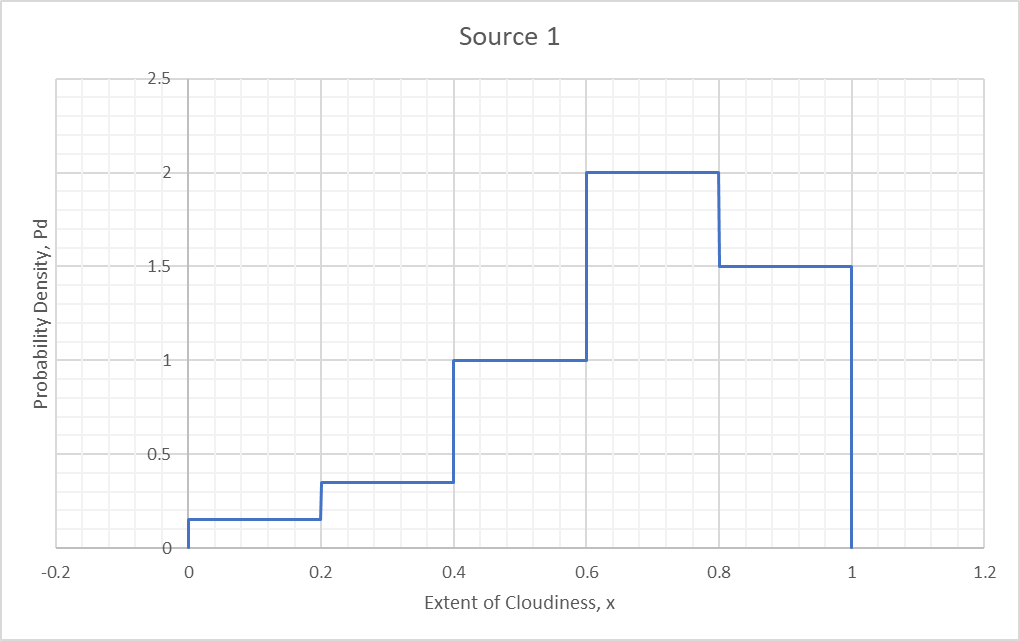
Our first source provides a distribution as follows:

This is a probability density function (PDF) and the total area under the curve is 1:

$$\int _{x=0}^{x=1}P_{d}dx=1$$

1 represents the total probability, ie that one of the outcomes in the distribution will happen. If we want to know the probability of an event lying between any two points on the x-axis, we write:

$$\int _{x=x_{0}}^{x=x_{1}}P_{d}dx=P$$

For example, the probability of overcast skies (0.6-0.8) is:

$$P_{overcast}=\int _{x=0.6}^{x=0.8}P_{d}dx=2(0.8-0.6)=0.4$$

For simple cases like this one where ${\textstyle P_{d}}$ is constant over some interval ${\textstyle x}$, ${\textstyle P=P_{d}\Delta x}$.

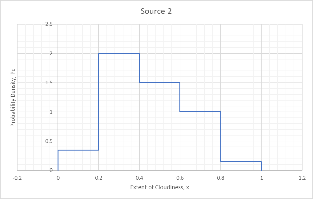
A second source produces the following distribution:

Our goal is to combine these sources via Bayes and the averaging techniques we have seen.

For the Bayesian combination we can write the combined probability density for an interval ${\textstyle x_{1}}$ to ${\textstyle x_{2}}$:

$$P_{comb,x_{1}tox_{2}}={{P_{d1,x_{1}tox_{2}}P_{d2,x_{1}tox_{2}}} \over {\int _{x=0}^{x=1}P_{d1}P_{d2}dx}}$$

For example, for the interval 0.6 to 0.8, the combined ${\textstyle P_{d}}$ is:

$$P_{comb,0.6to0.8}={2(1) \over {0.2(0.15)(0.35)+0.2(0.35)(2)+0.2(1)(1.5)+0.2(2)(1)+0.2(1.5)(0.15)}}=2.23$$

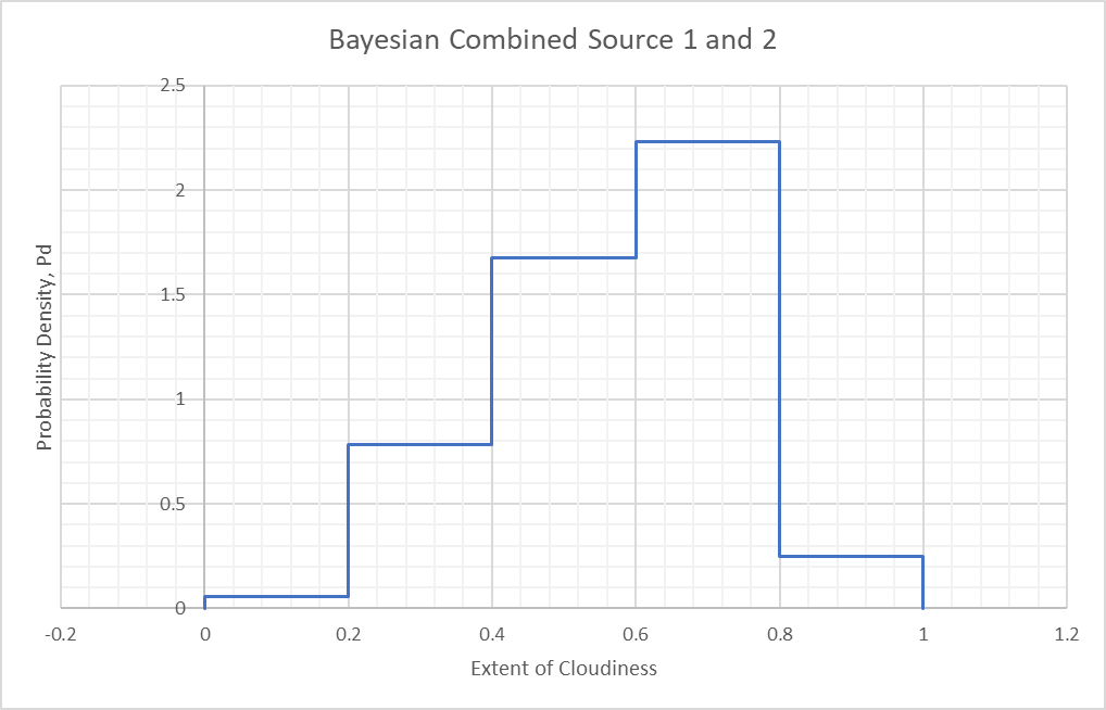
Doing this for each interval and plotting the results leads to the following graph of combined ${\textstyle P_{d}}$:

This graph can then be used as the updated distribution to which new source distributions can be combined in exactly the same manner. In general we see that combining distributions is no different than using the Bayes equation as we have, except that we have more sub-intervals to consider and the denominator is an integral rather than a summation of probability products.

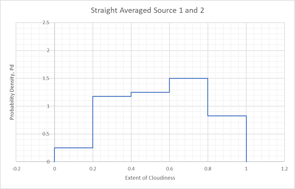
Averaging or trust-weighted averaging works exactly the same way: each sub-interval is taken and averaged to produce a new distribution. A straight average of the overcast case above leads to:

$$P_{d,ave,overcast}={P_{d1,0.6to0.8}+P_{d2,0.6to0.8} \over 2}={{2+1} \over 2}=1.5$$

Doing this for each subinterval leads to the following distribution:

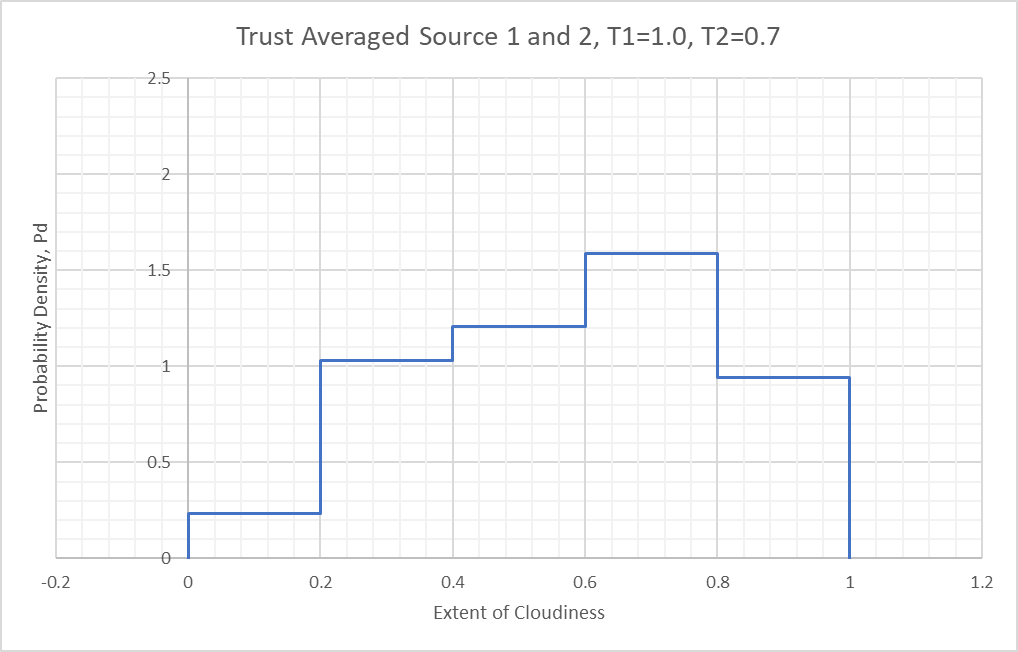
Trust weighted averaging also works the way you’d expect, with each sub-interval handling the trust-weighting and averaging scheme. Again, for the 0.6 to 0.8 sub-interval, assuming a Trust=1.0 for the 1st source and a Trust=0.7 for the 2nd Source:

$$P_{d,tave,overcast}={T_{1}P_{d1,0.6to0.8}+T_{2}P_{d2,0.6to0.8} \over {T_{1}+T_{2}}}={{1(2)+0.7(1)} \over {1+0.7}}=1.588$$

Doing this over each sub-interval and plotting leads to:

This Excel spreadsheet (Sheet 1), binning.xlsx , and snippet reproduce the calculations shown here.

Continuous Distributions

The above situation was a semi-continuous distribution, piecewise if you will. For the case of a fully continuous distribution, where the source provides a function, we can largely approach it the same way, by breaking up the function into discrete sub-intervals and performing numerical integration.

Let’s suppose Source 1 answers the question with a Weibull distribution:

$$P_{d1}={k \over \lambda }{\left({x \over \lambda }\right)}^{k-1}e^{-\left({x \over \lambda }\right)^{k}}$$

Where:

${\textstyle k=7}$ (known as a “shape” parameter)

${\textstyle \lambda =0.7}$ (known as a “scale” parameter)

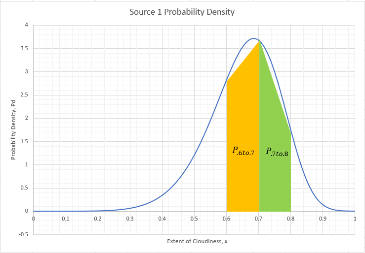
However, it is not important what the functional form of the distribution is (this is just an example) as long as the area under the curve is 1. If we plot this distribution we obtain:

As we saw above, the probability of the cloudiness extent being in any given sub-interval is the area under the curve of that sub-interval. We obtain the area by integrating numerically. If we break up the function into 10 equally spaced sections we can find the area for the sub-interval x=0.6 to 0.8 by adding the areas for the sections 0.6 to 0.7 (yellow region) and 0.7 to 0.8 (green region):

$$P_{0.6to0.8}=\int _{x=0.6}^{x=0.8}P_{d1}(x)dx\approx 0.5(P_{d1.6}+P_{d1.7})(\Delta x)+0.5(P_{d1.7}+P_{d1.8})(\Delta x)$$

$$=0.5(2.8229+3.6788)(0.1)+0.5(3.6788+1.7459)(0.1)=0.5963$$

This area is not very accurate because we only used 10 sections. But if we break the function up into more sections (ie make ${\textstyle \Delta x}$ small enough) we can obtain an accurate approximation of the area. We can then sum these small areas to find the area for any reasonably sized sub-interval.

Note that we are using trapezoidal areas here rather than the simple rectangular areas used in the binned example. This is only for the purpose of numerical accuracy. We could have used rectangular areas but then we would require more sections (a finer grid), and hence more computation, to achieve good accuracy.

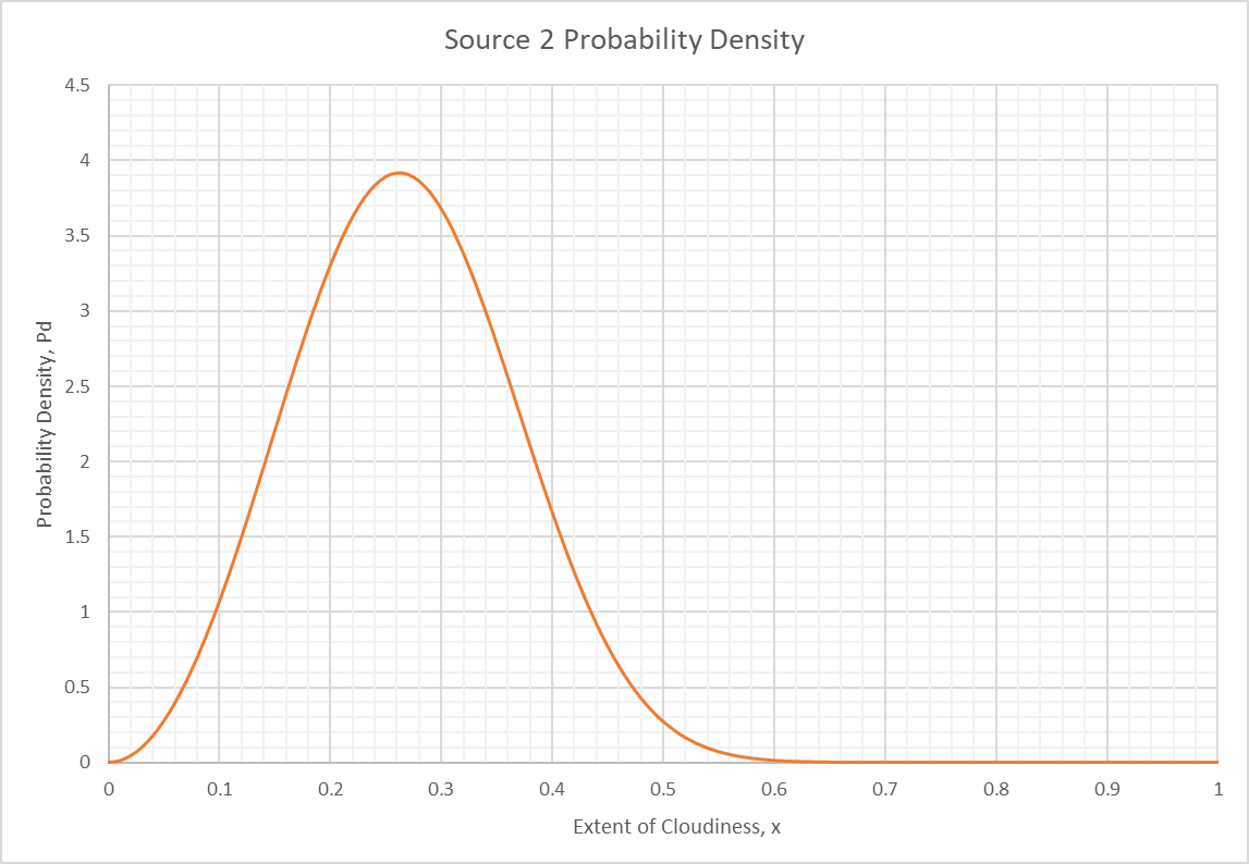
Let’s introduce a 2nd source who answers the question with a 2nd Weibull distribution but shaped and scaled a little differently:

${\textstyle k=3}$ (“shape” parameter)

${\textstyle \lambda =0.3}$ (“scale” parameter)

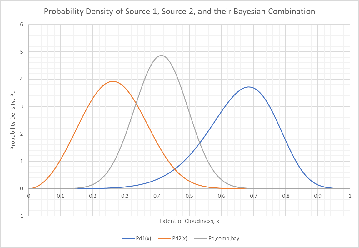
Source 2 believes the weather tomorrow will be sunnier than Source 1. To combine these distributions via Bayes, we write:

$$P_{d,comb,bay,x_{1}tox_{2}}={{P_{d1,x_{1}tox_{2}}P_{d2,x_{1}tox_{2}}} \over {\int _{x=0}^{x=1}P_{d1}P_{d2}dx}}$$

The numerator is just the product of ${\textstyle P_{d}}$ for each source at the desired ${\textstyle x}$. The denominator is the area under the curve of a function comprising the product of ${\textstyle P_{d1}}$ and ${\textstyle P_{d2}}$. This area is found by integrating numerically using the same technique as above (with trapezoidal sections):

$${\int _{x=0}^{x=1}P_{d1}P_{d2}dx}\approx \sum _{i=1}^{n}0.5\lbrack P_{d1}P_{d2}(x_{min}+(i-1)\Delta x)+P_{d1}P_{d2}(x_{min}+i\Delta x)\rbrack \Delta x$$

where

${\textstyle n}$ is the number of sections (=10 for example)

${\textstyle x_{max}}$ is the maximum value of ${\textstyle x}$ (=1 in this case)

${\textstyle x_{min}}$ is the minimum value of ${\textstyle x}$ (=0 in this case)

${\textstyle \Delta x={x_{max}-x_{min} \over n}}$

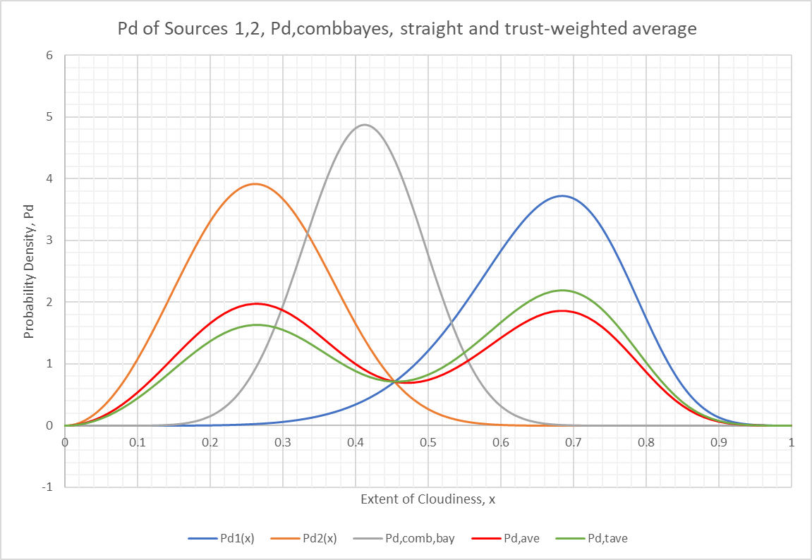
If we do this for all ${\textstyle n}$ sections we can plot the results along with the ${\textstyle P_{d}}$ for the first two sources for comparison.

We can calculate the straight average at ${\textstyle x=0.6}$ (for example) and obtain:

$$P_{d,ave}={P_{d1,x=.6}+P_{d2,x=.6} \over 2}={{2.823+.0134} \over 2}=1.418$$

For the trust-weighted average with ${\textstyle T_{1}=1.0}$ and ${\textstyle T_{2}=0.7}$ also at ${\textstyle x=0.6}$ we have:

$$P_{d,tave}={1.0(P_{d1,x=.6})+0.7(P_{d2,x=.6}) \over 1+0.7}={{2.823+0.7(.0134)} \over 1+0.7}=1.666$$

If we do these averages for several points, we can add the resulting plot to the plot above:

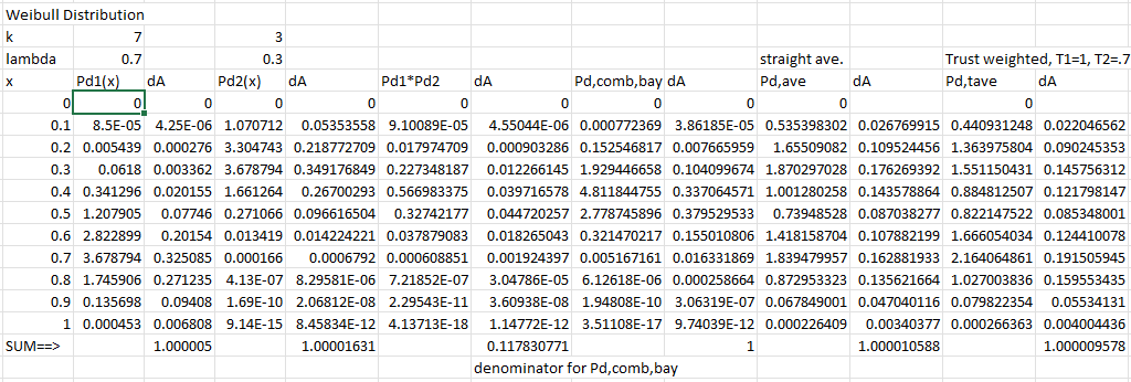
A table of the values used for the case ${\textstyle n=10}$ is shown here:

The curves above were actually plotted for ${\textstyle n=100}$ but the values at the points shown in this table correspond quite closely. An Excel spreadsheet to do the calculations is here (Sheet 2): binning.xlsx

Now, to find the probability of any sub-interval within any of these combined curves, we numerically integrate as shown above for Source 1. This is equivalent to adding up each section’s area, the dA values shown in the table & spreadsheet above.

For the case of Source 1 between ${\textstyle x=0.6}$ and ${\textstyle x=0.8}$ we have:

$$P_{1,0.6to0.8}=0.325085+0.271235=0.5963$$

This, you will notice, is the same value as that produced above when we performed the numerical integration “from scratch”.

For Source 2, we have:

$$P_{2,0.6to0.8}=0.0006792+8.29581(10)^{-6}=0.000687496$$

For the Bayesian combination we have:

$$P_{bay,0.6to0.8}=0.01633+0.000258=0.01659$$

and so on. The numbers above refer to the ${\textstyle n=10}$ case. We can perform these calculations for all the curves for ${\textstyle n=10}$ and ${\textstyle n=100}$ (values in the Excel spreadsheet) and produce the following table:

We can see that Source 1 believes, to a large extent, in overcast skies tomorrow. Source 2, however, doesn’t believe that at all. The Bayesian combination, as it tends to do, pulls in favor of certainty so produces a low probability of overcast skies. The average produces something in between and the trust weighted average favors Source 1 a little because it discounts Source 2 somewhat (Trust = 0.7).

Also notable is the fact that we obtain a small but significant change in the values as we move from ${\textstyle n=10}$ to ${\textstyle n=100}$. It isn’t clear from this that we have achieved “grid independence” but we are very close. Grid independence means that refining the calculation with more steps does not lead to improved accuracy, indicating that the number of steps we have is correct. This snippet, which reproduces the calculations above, can be run at ${\textstyle n=1000}$ and you will see that the answers don’t change much. We should be careful to refine the grid only when necessary because it increases the cost of calculation enormously.

Summary

The key point in all this analysis is that the math we’ve developed so far applies to probability densities in exactly the same way as it does for simple probabilities. There’s just more of it because you have to break up the distribution into small increments along the x axis and do the math on each increment. But the math is the same.

We’ve covered three possibilities so far for how respondents can answer questions: 1) They can assign a single probability to their answer, 2) They can provide a binned distribution, and 3) they can provide a truly continuous distribution. They can also just answer the question without giving a probability but this is a special case of 1 where we assume a probability of 100%.

It is likely that 1 and 2 will be the preferred ways to answer. The continuous distribution, although important, seems like the vicinity of experts who perform a study or simulation to come up with their function.

Also, keep in mind that continuous distributions are only useful in cases where there is a continuous variable. The binned distribution can be used even when there isn’t a continuous variable because, for truly discrete categories, you can simply break up the x-axis into equal length sections and use the same math. This is what Sapienza did, for instance. You can also just dispense with the x-axis and use the probabilities (instead of probability densities), as we’ve been doing in the work before this post.

This brings up the question of why Sapienza chose to use a binned distribution for what was, at first glance, a discrete variable problem. One answer is that maybe he meant for his example to represent a continuous variation from good to bad weather. For simplicity, he then broke up the x-axis into equal length bins. It is certainly easier to think about continuous variations as a collection of discrete groupings. But the more likely explanation is that he did it because it is a more generalized method that works for all cases, discrete and continuous.